Optimization#
- find_optimal(fsm: FisherModel, optimization_strategy: str = 'scipy_differential_evolution', discrete_penalizer='default', verbose=True, **kwargs)#
Find the global optimum of the supplied FisherModel.
- Parameters:
fsm (FisherModel) – The FisherModel object that defines the studied system with its all constraints.
optimization_strategy (str) –
Choose the optimization strategy to find global maximum of the objective function. The default is “scipy_differential_evolution”.
- ”scipy_differential_evolution” (recommended)
The global optimization method uses the scipy.optimize.differential_evolution function showing rather good results for nonlinear dynamic problems. The strategy was developed by Storn and Price (1996) and work as follows.
Firstly, the initial population of the vectors of all optimized values (times and inputs) for one Experimental Design (solutions) is randomly chosen from the region of available values. Then each solution mutates by mixing with other candidates. To a chosen one solution from the initial population \(D_0\), a weighted difference between two other random solutions from the same set \((D_\text{rand1} - D_\text{rand2})\) is added. This process is called mutation and a new vector \(D_m\) is obtained. The next step is to construct a new trial solution. This is done by randomly choosing the elements of this vector either from the initial \(D_0\) or the mutated \(D_m\) solutions. For each new element of trial vector, from the segment [0, 1) the number should be randomly picked and compared to the so-called recombination constant. If this number is less than a constant, then the new solution element is chosen from mutated vector \(D_m\), otherwise from \(D_0\). So, in general, the degree of mutation can be controlled by changing this recombination constant. When the trial candidate is built, it is compared to initial solution \(D_0\), and the best of them is chosen for the next generation. This operation is repeated for every solution candidate of the initial population, and the new population generation can be formed. The process of population mutation is repeated till the desired accuracy is achieved. This method is rather simple, straightforward, does not require the gradient calculation and is able to be parallelized.
- ”scipy_basinhopping”
The global optimization method uses the scipy.optimize.basinhopping function. The algorithm combines the Monte-Carlo optimization with Methropolis acceptance criterion and local optimization that works as follows. The strategy is developed by David Wales and Jonathan Doye and combines the Monte-Carlo and local optimization. The classic Monte-Carlo algorithm implies that the values of the optimized vector are perturbed and are either accepted or rejected. However, in this modified strategy, after perturbation, the vector is additionally subjected to local optimization. And only after this procedure the move is accepted according to the Metropolis criterion.
- ”scipy_brute”
The global optimization method uses the scipy.optimize.brute function. It is a grid search algorithm calculating the objective function value at each point of a multidimensional grid in a chosen region. The technique is rather slow and inefficient but the global minimum can be guaranteed.
discrete_penalizer (str) –
A function that takes two 1d arrays (values, discretization) and returns a float. It calculates the penalty (1=no penalty, 0=maximum penalty) for datapoints which do not sit on the desired discretization points.
- ”default”
Uses the default penalty function that is described by the function
discrete_penalty_calculator_default().
- ”product_difference”
Uses the discretization penalty function described by the function
discrete_penalty_calculator_default().
- ”individual_zigzag”
Uses the discretization penalty function described by the function
discrete_penalty_individual_template()with the penalty structure pen_structure=penalty_structure_zigzag.
- ”individual_cos”
Uses the discretization penalty function described by the function
discrete_penalty_individual_template()with the penalty structure pen_structure=penalty_structure_cos.
- ”individual_gauss”
Uses the discretization penalty function described by the function
discrete_penalty_individual_template()with the penalty structure pen_structure=penalty_structure_gauss.
- Raises:
KeyError – Raised if the chosen optimization strategy is not implemented.
- Returns:
The result of the optimization as an object FisherResults. Important attributes are the conditions of the Optimal Experimental Design times, inputs, the resultion value of the objective function criterion.
- Return type:
- display_optimization_end(fsr: FisherResults)#
- display_optimization_start(fsmp: FisherModelParametrized)#
- class PenaltyInformation(penalty: float, penalty_ode_t0: float, penalty_inputs: float, penalty_times: float, penalty_summary: dict)#
Bases:
object- penalty: float#
- penalty_inputs: float#
- penalty_ode_t0: float#
- penalty_summary: dict#
- penalty_times: float#
- discrete_penalty_calculator_default(vals, vals_discr)#
The discretization penalty function taken as a product of all differences between the optimized value \(v\) and all possible discrete values allowed \(v^{\text{discr}}\). If there is no penalty, a function gives 1 and 0 in case of the maximum penalty for data points that do not sit on the desired discretization points.
\[U_1(v) = 1 - \sqrt[N]{\prod_{k=1}^N (v - v^{\text{discr}}_{k})} \frac{1}{\max(v^{\text{discr}}) - \min(v^{\text{discr}})},\]where \(N\) is the size of the vector of the allowed discrete values \(v^{\text{discr}}\). The resulting contribution of the penalty function is a product of the potential values for each value \(v\).
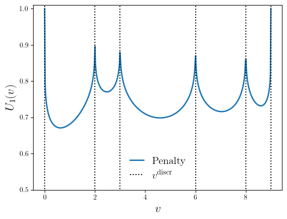
The discretization penalty function for discrete values \(v^{\text{discr}} = [1, 2, 3, 6, 8, 9]\).#
The resulting contribution of the penalty function is calculated as a product of all penalty values for each value \(v\).
\[U = \prod_{i=1} U_1(v_i).\]- Parameters:
vals (np.ndarary) – The array of values to optimize \(v\).
vals_discr (np.ndarary) – The array of allowed discrete values \(v^{\text{discr}}\).
- Returns:
The array of the penalty potential values for vals. The resulting contribution (product) of the penalty function.
- Return type:
np.ndarary, float
- discrete_penalty_individual_template(vals, vals_discr, pen_structure)#
The discretization penalty function template. If there is no penalty, a function gives 1 and 0 in case of the maximum penalty for data points that do not sit on the desired discretization points.
The resulting contribution of the penalty function is calculated as a product of all penalty values for each value \(v\).
\[U = \prod_{i=1} U_1(v_i).\]- Parameters:
vals (np.ndarary) – The array of values to optimize \(v\).
vals_discr (np.ndarary) – The array of allowed discrete values \(v^{\text{discr}}\).
pen_structure –
Define the structure of the template.
penalty_structure_zigzag()Use zigzag structure.
penalty_structure_cos()Use cosine function for potential.
penalty_structure_gauss()Use two Gaussian functions.
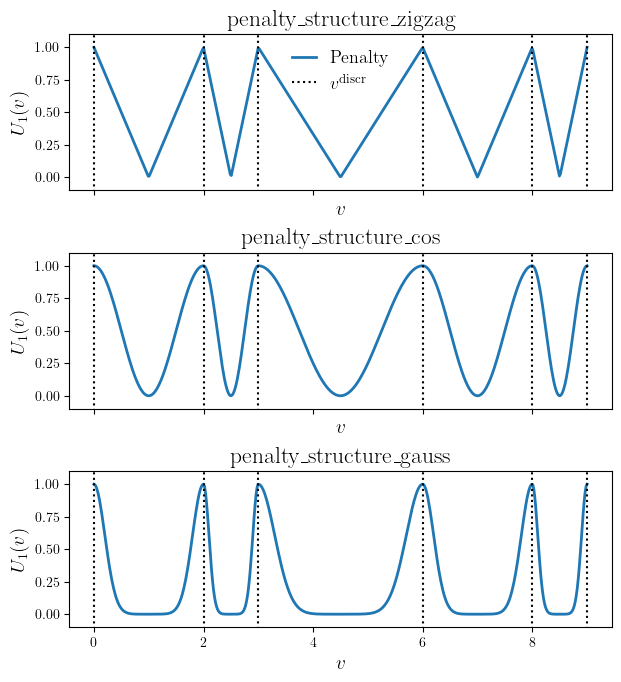
The discretization penalty function for discrete values \(v^{\text{discr}} = [1, 2, 3, 6, 8, 9]\) for different penalty structures.#
- Returns:
The array of the penalty potential values for vals. The resulting contribution (product) of the penalty function.
- Return type:
np.ndarary, float
- penalty_structure_cos(v, dv)#
Define the cosine structure of the penalty potential between two allowed discrete values described by equation
\[U_1(v) = \frac{1}{2} (1 + \cos{2 \pi v}),\]where \(v\) is the distance between the optimized value and the smaller neighboring discrete value and \(dv\) is the distance between smaller and larger neighboring discrete values. The function is used as an argument in function
discrete_penalty_individual_template()and dtermines the shape of it.- Parameters:
v (float) – The distance between the optimized value and the smaller neighboring discrete value \(v\).
dv (float) – The distance between smaller and larger neighboring discrete values \(dv\).
- Returns:
The value of the penalty potential.
- Return type:
float
- penalty_structure_gauss(v, dv)#
Define the gaussian structure of the penalty potential between two allowed discrete values described by equation
\[U_1(v) = e^{-\frac{v^2}{2\sigma^2}} + e^{-\frac{(v-dv)^2}{2\sigma^2}}\]where \(v\) is the distance between the optimized value and the smaller neighboring discrete value, \(dv\) is the distance between smaller and larger neighboring discrete values and the variance is \(\sigma = 0.1dv\). The function is used as an argument in function
discrete_penalty_individual_template()and dtermines the shape of it.- Parameters:
v (float) – The distance between the optimized value and the smaller neighboring discrete value \(v\).
dv (float) – The distance between smaller and larger neighboring discrete values \(dv\).
- Returns:
The value of the penalty potential.
- Return type:
float
- penalty_structure_zigzag(v, dv)#
Define the zigzag structure of the penalty potential between two allowed discrete values described by equation
\[U_1(v) = \bigg|1 - \frac{2 v}{dv}\bigg|,\]where \(v\) is the distance between the optimized value and the smaller neighboring discrete value and \(dv\) is the distance between smaller and larger neighboring discrete values. The function is used as an argument in function
discrete_penalty_individual_template()and dtermines the shape of it.- Parameters:
v (float) – The distance between the optimized value and the smaller neighboring discrete value \(v\).
dv (float) – The distance between smaller and larger neighboring discrete values \(dv\).
- Returns:
The value of the penalty potential.
- Return type:
float